Abstract

A number of new features have been added to Visualyse Professional during 2017 to support the modelling of 5G / IMT-2020 systems, in particular the beamforming antennas, wanted signal path loss models, clutter loss models, UE deployment models and the TDD traffic model. A recent Technical Note (TN) showed how to use these features to create a simulation with a single BS and three UEs. Often, however, scenarios involve the deployment of large numbers of co-frequency 5G / IMT-2020 systems, more than can be readily modelled using standard techniques. This TN shows how a reference system approach can be used to model the behaviour of a single cell via an aggregate EIRP CDF (AEIRP). This AEIRP CDF can then be readily re-used over many cells to create an interference scenario involving widescale deployments. This approach could be used in other scenarios with large numbers of interferers, including as 4G mobile or RLANs.

Overview

Transfinite has been working on a series of upgrades to Visualyse Professional to include the features needed to model 5G / IMT-2020 systems. There has also been an increasing degree of agreement at international groups as to the parameters and scenarios.

A previous TN shows step by step how to use Visualyse Professional to build a single sector 5G system for urban environments in the 26 GHz band, including comparison of the results with other implementations.

One of the characteristics of 5G / IMT-2020 systems is that they are expected to operate over short distances and could have high deployment densities (e.g. in urban areas). This has implications on how the scenarios are to be modelled, for example consider:

• A fixed service receiver co-frequency with a 5G / IMT-2020 deployment, with the requirement to identify the minimum exclusion zone around it required to avoid harmful interference
• A GSO satellite receiver co-frequency with 5G / IMT-2020 deployed across a large area such as continent, to study if sharing is feasible.

The common factor in both of these scenarios is that there could be large numbers of interfering systems - potentially millions - to be considered. This would be too large for each BS and UE to be modelled individually and techniques must be employed to simplify the modelling without significant loss of accuracy.

One such approach is the concept of the "reference system" as described in this document: this could be combined with other approaches such as increasing the power by $10 \log _{10} \mathrm{N}$ where N is the number of stations.

Modelling Using Reference Systems

The idea about using a reference systems is to split the modelling into two stages:

1. Model in detail all the emissions from all the transmitters in a given square area with side d, and calculate the aggregate equivalent isotropically radiated power (AEIRP). Using Monte Carlo methods, randomise the inputs (e.g. UE location, cell orientation, propagation model, traffic etc.) to generate a cumulative distribution function (CDF) of the AEIRP.
2. Model the deployment of cells across a larger area via a set of stations, each representing all transmitters in a d x d area. The EIRP of each of these reference stations can then be modelled by sampling from the AEIRP CDF calculated in stage 1. This can then be used with appropriate propagation model(s) to calculate the interference into a victim system.

This approach is shown in the figures below:

Stage 1: Creating the AEIRP CDF

Stage 2: Using the AEIRP CDF

This approach has been documented in the following two ITU-R Recommendations:

• F.1760: Methodology for the calculation of aggregate equivalent isotropically radiated power (a.e.i.r.p.) distribution from point-to-multipoint high-density applications in the fixed service operating in bands above 30 GHz identified for such use
• F.1766: Methodology to determine the probability of a radio astronomy observatory receiving interference based on calculated exclusion zones to protect against interference from point-to-multipoint high-density applications in the fixed service operating in bands around 43 GHz

While these are F-series recommendations (i.e. for the Fixed Service) the methodology is applicable for many other service types and scenarios.

This approach tends to be more accurate when there would be little variability in the interferer propagation loss across the reference system’s area. Hence the distance d should be significantly less than distance from any of the interfering reference system to the victim station.

Also, if terrain were used for the second stage, then there is the danger of underestimating interference as the reference station might not be located at the point with the lowest propagation loss towards the victim. This can be voided by locating the reference station at the highest point within the d x d area.

AEIRP Equations

The interference calculation for a single interferer is typically similar to this:

$$I_i=P_{t x, i}+G_{t x, i}-L_{p a t h, i}-L_{c l u t t e r, i}+G_{r x, i}$$

When there are N transmitters the aggregate interference can be calculated using the summation:

$$I_{\text {agg }}=10 \log \left[\sum_{i=1}^{i=N} 10^{\frac{I_i}{10}}\right]$$

In scenarios where all parameters are the same for N stations, the aggregation can be modelled using a single station and increasing the transmit power by $10 \log _{10} N$. If that is not the case, then a more flexible approach is to use a reference system. The reference system approach assumes that the N transmitters are in an area (e.g. $d \times d \mathrm{~km}$ ) that is sufficiently small compared to the separation between them and the receiver that the following terms are approximately the same over all of them:

$$L_{p a t h, i}+G_{r x, i}$$

Hence interfering calculation becomes:

$$I_{\text {agg }}=A E I R P-L_{p a t h}+G_{r x}$$

Where:

$$A E I R P=10 \log \left[\sum_{i=1}^{i=N} 10^{\frac{E I R P_i}{10}}\right]$$

And:

$$\operatorname{EIRP}_i=P_{t x, i}+G_{t x, i}-L_{c l u t t e r}, i$$

Note that in this case the AEIRP includes the clutter at the transmitter end. It could also assume no clutter or also include building entry loss. There could also be clutter at the victim end, which would be added to the $I_{\text {agg }}$ calculation rather than the AEIRP calculation. The equations above show a single value of $I_{\text {agg }}$ and AEIRP, but in general these terms will also vary in the time domain and hence be represented by distributions i.e. via a CDF.

Deployment vs. Time Domains

Monte Carlo analysis can be used to model variations in two very different domains:

• Variations in the deployment domain (for example, the location of the BS or physical pointing of the its antenna)
• Variations in the time domain (for example, location of the UE or traffic direction DL/UL).

These are two different domains and it can be dangerous to convolve the two together in a single Monte Carlo simulation.

In particular, if a BS is deployed with a specific geometry it will be fixed for all time.

For example, consider an interfering path from BS to victim satellite ES and the two geometries shown below:

Geometry 1: BS pointing away from ES and clutter between BS and ES

Geometry 2: BS pointing towards the ES and line of sight between BS and ES:

In the first case there is clutter loss between the BS and the ES and at 26 GHz this is likely to represent a significant attenuation of the interfering signal.

In the second case there is direct line of sight between the BS and the ES and so the interfering signal will be much stronger.

As the BS deployment is static this can result in significant variation in the levels of interference. In both cases there would be time variation (e.g. due to traffic, other propagation effects and UE location) but there would be a significant difference in the CDF of the I/N at the ES.

The approach to take depends upon the relative distance from the nearest BS to the ES:

• If there is a short distance between the nearest BS and the ES or small number of interferers, then the aggregate interference could be driven by a single interferer and hence the deployment of that particular station will be key.

  In this case it might be better to define a set of specific scenarios that model the environment around the ES, for the reality is that results will be dependent upon the deployment geometry.

• If there is a large distance between the nearest BS and the ES and large numbers of interferers, then there is likely to be a greater difference between the worst single interferer and the aggregate interference, and hence less impact from the deployment of any specific station.

With large numbers of BS it is more likely that the deployment distribution would match that of a randomised deployment, and hence it can be acceptable to convolve the two together.

Building the Single Cell Sim

The previous TN, “Building a 5G Network in Visualyse Professional” showed how to create a single cell 5G / IMT-2020 system based upon the following documents:

• Recommendation ITU-R M.2101: Modelling and simulation of IMT networks and systems for use in sharing and compatibility studies
• Working Party 5D Attachment 2 on Spectrum Needs to a liaison statement to TG 5/1: Characteristics of terrestrial IMT systems for frequency sharing / interference analysis in the frequency range between 24.25 GHz and 86 GHz
• Annex 1 to Document 5-1/92-E Task Group 5/1 Chairman’s Report: System parameters and propagation models to be used in sharing and compatibility studies
• Section 4.17 of Document 5D/666 Chairman’s Report: Example implementation of the methodology in Recommendation ITU-R M.2101

This simulation file is available on request.

Building the Reference System

The result of the previous TN was a simulation file that modelled a single sector BS pointing east providing communication services to 3 UEs. To calculate the AEIRP CDF the following changes were made:

1. Randomise the azimuth of the sector to model the variation in AEIRP due to the relative geometry
2. Include a TDD model of activity of the three links
3. Include a test station to detect the AEIRP with isotropic antenna
4. Set the propagation loss for the interfering path to be zero + clutter loss so that the aggregate interference into this test station is the AEIRP after including clutter at the transmitter
5. Create a RX link at the test station on 26 GHz with bandwidth = carrier = 180 MHz
6. Create an interference path from the three BS to UE links to this new RX link
7. Configure the statistics and Monte Carlo samples to get the required outputs.

These changes are described below.

Randomize the BS Orientation

The BS azimuth can be randomized in Visualyse Professional easily as it just requires a single parameter to be changed, as highlighted in the screenshot below:

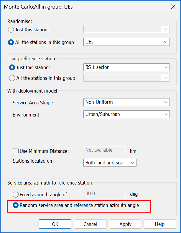
As noted above, this results in variation in both the time and deployment domains.

Include a TDD Model

It is proposed that 5G / IMT-2020 systems will use time division duplex (TDD) to communicate between the BS and UE. This can be modelled by creating a traffic object in Visualyse Professional and configuring for the TDD model with parameters as in the dialog below:

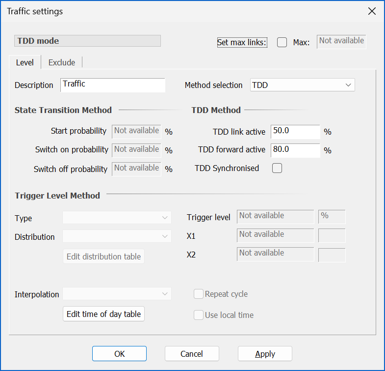
This shows the relevant parameters which are:

• Activity: 50% of the time (20% could also be considered)
• Direction: 80% of the time in the DL direction.

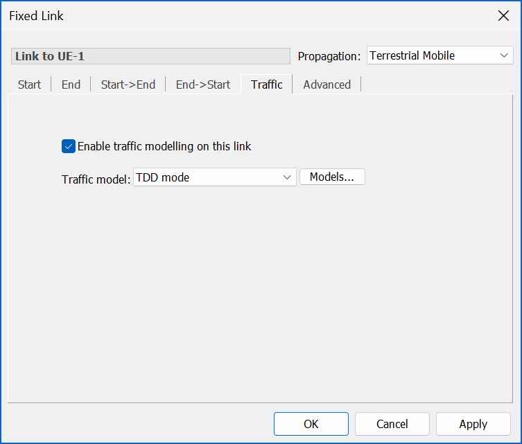
This model can then be associated with each of the three links on their Traffic tab as per the figure below:

Create a Test Station

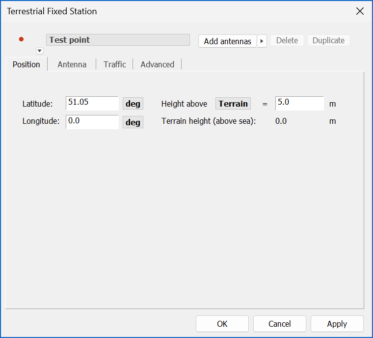
The test station should be created with similar geometry to the resulting victim station used in stage 2.

So if the use is for a terrestrial path it should be at the same height as the intended victim, located sufficiently far away that it appears on the horizon as seen by the BS (so that the gain calculated is the gain towards the horizon) as in the following dialog:

If the use is for a satellite path it should be at the relevant orbit height e.g. GSO and having the required elevation angle.

Set the Propagation Model

As described above in the section on the equations, the propagation model should be set to a core path loss of 0 dB plus including clutter loss at the transmitter side.

Hence the propagation environment should look like this:

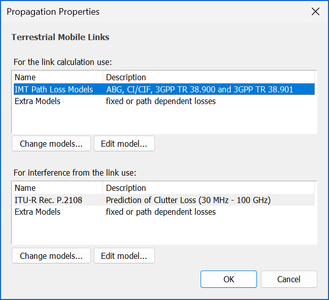
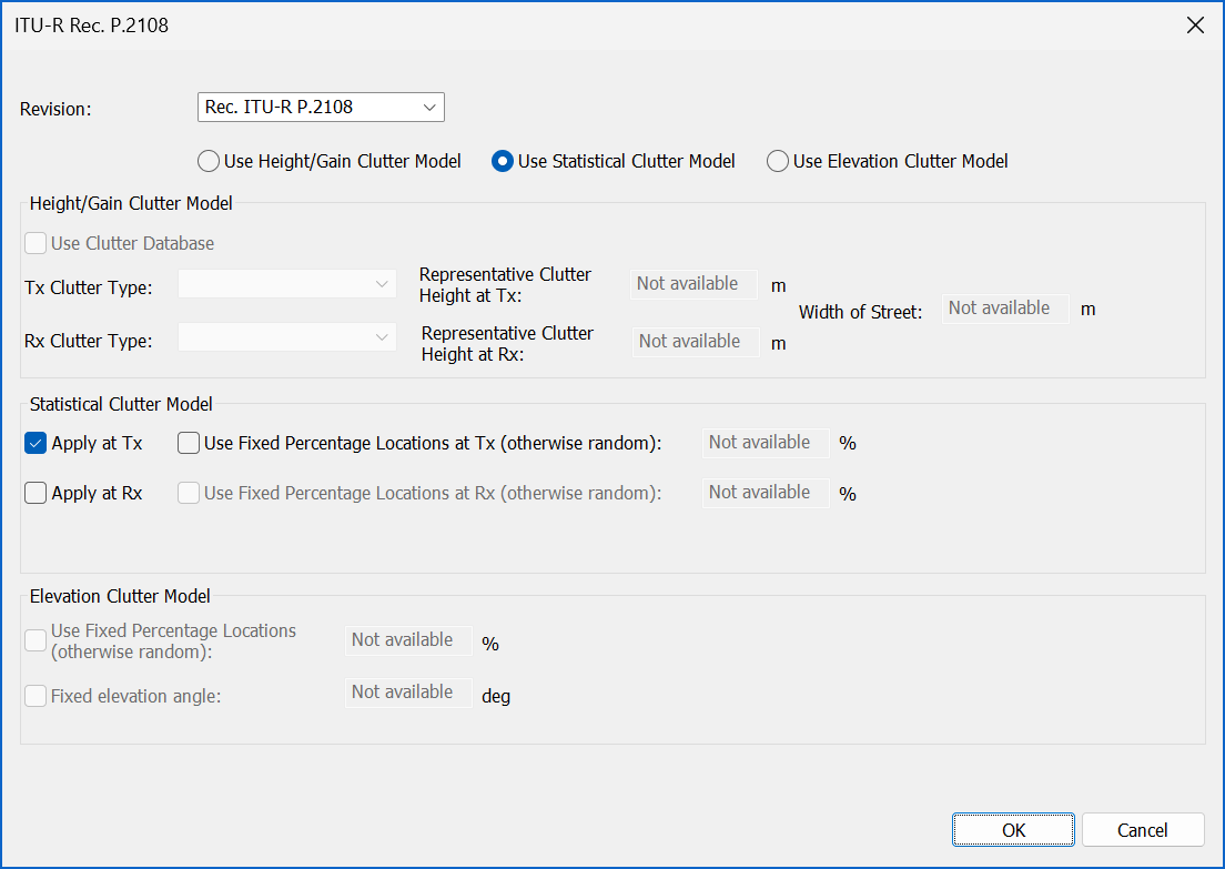
The extra loss is simply zero while the P.2108 is configured to be the statistical model considering a random loss at the transmit side, as per the following:

Creating the RX Link

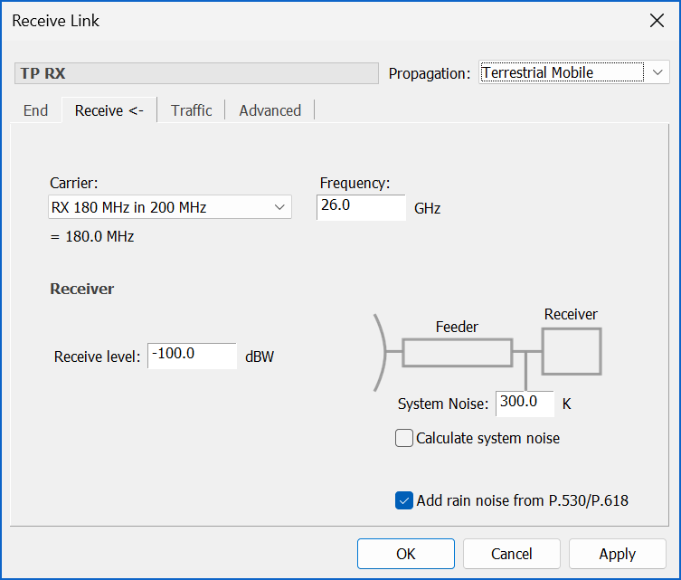
The first step to create the RX link is to create a carrier with bandwidth 180 MHz. This was selected as it covers all three of the BS to UE carrier frequencies. This will also be reference bandwidth associated with the AEIRP CDF.

The 180 MHz carrier can then be used for a receive link centered on 26 GHz using the test station created previously, with link path tab as in the figure below:

Interference Path

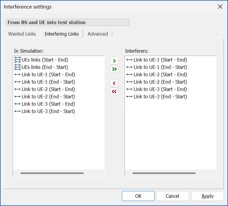
An interference path can then be created with:

• Victim / Wanted link: TP RX link
• Interfering links: the 3 BS to UE links, both the start->end and end->start directions, as in the figure below:

The other settings can be left unchanged.

Configure the Simulation

The final steps are to configure the simulation by:

• Setting the number of Monte Carlo samples used to generate the AEIRP CDF: in this case 10,000 time steps were used
• Setting the statistics option to gather I statistics and also the histogram with bin size 0.1 dB.

Checking the Simulation

As always it is important to check the simulation is working as expected. In this case a good check is that the worst single entry interfering link budget is effectively an EIRP, and the number of interferers is consistent with the number of UEs and TDD traffic option.

The can be seen by configuring a watch window as in the figure below.

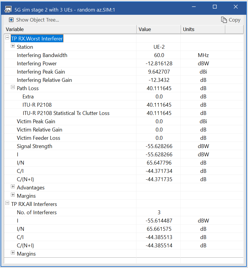
Note that the values could be different depending upon the random number sequence on your PC.

If you run this simulation interactively these numbers should update and:

• The number of interferers should vary in accordance with the traffic module
• The sector azimuth of the BS should change to be pointing in any direction with equal likelihood
• The location of the UE within the sector should be selected at random using the non-uniform density
• Hence the gain at the BS and UE towards the test point should change at each sample
• The UE transmit power is likely to vary due to the gain patterns and propagation model characteristics
• The clutter loss is likely to vary according to the statistical model.

An example screenshot is shown below including a CDF of the AEIRP as calculated after 10,000 samples:

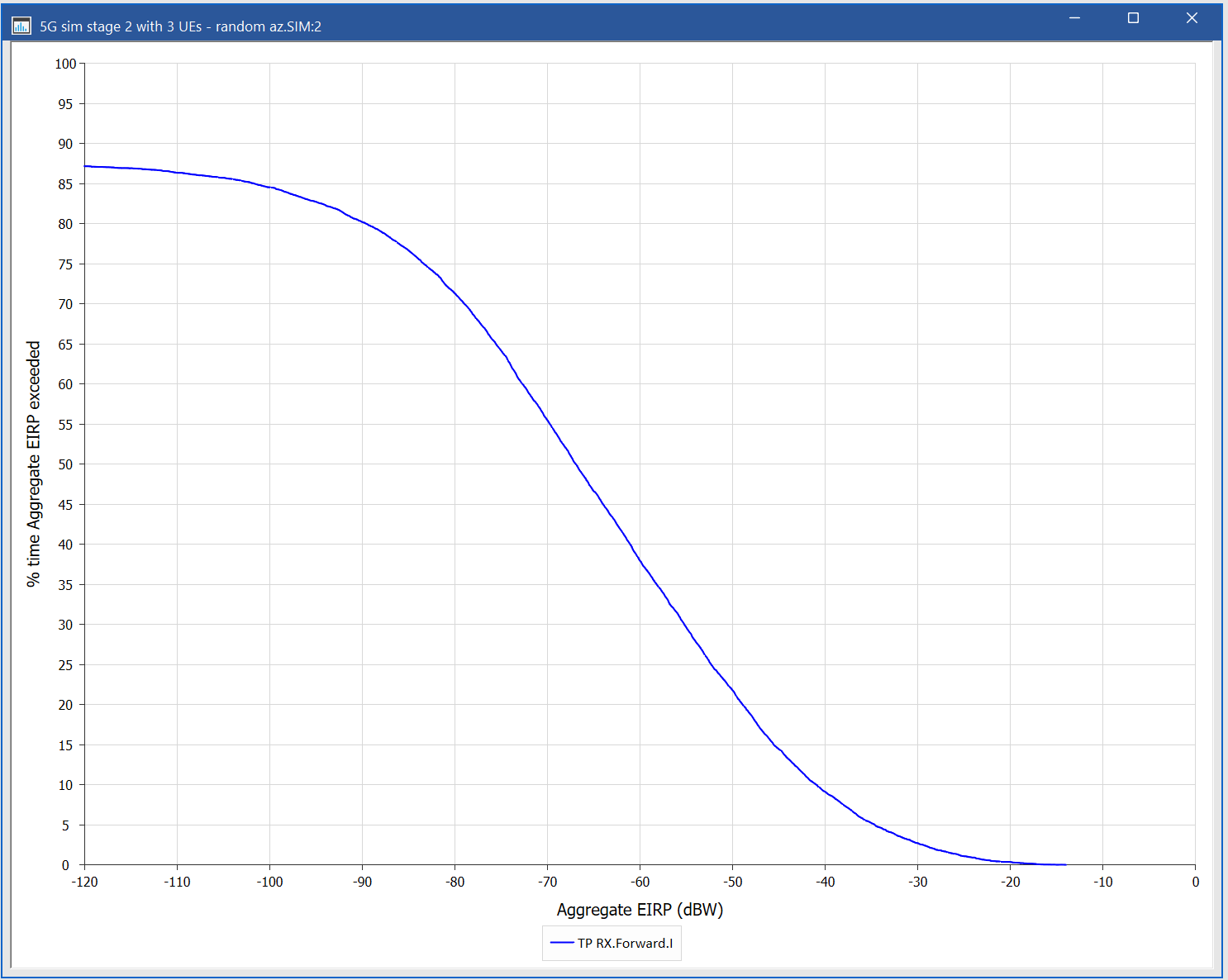
Note that the AEIRP CDF does not go all the way up to 100%: this is because the likelihood that each link is active is 50% and hence not active 50%. The probability that all three links are not active is therefore (1/2)$^3$ or 12.5%. Hence the time that at least one link is active is 87.5%.

Converting the Output into an Input

The next stage is convert the output from the stage 1 simulation into an input to the stage 2 simulation file. These are:

• Outputs from Stage 1: CDF of the AEIRP. This can be extracted by looking at the Results | View Results dialog for the RX link’s I statistics, which will show the histogram (see below)

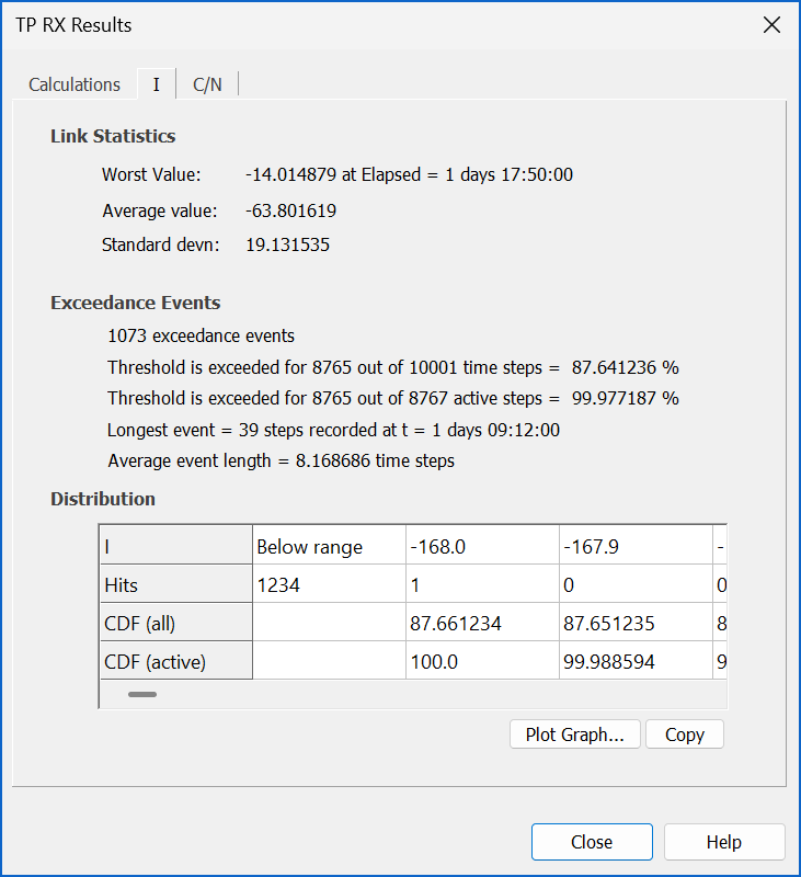
• Inputs into Stage 2: This will be a CDF of the AIERP in the format of a table [p, AEIRP(p)] to be used by a Monte Carlo define variable.

It will be necessary to convert these format, and this can readily be done using a tool such as Excel.

From:

To:

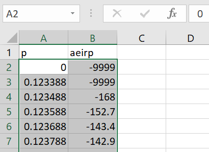
This is the format that will be used as the input to the second stage simulation.

Using the AEIRP CDF

Having created the AEIRP CDF it can be used in the second stage simulation.

This requires:

• Antenna type: with an isotropic / omni gain pattern
• Station: using the isotropic antenna and with the the same height as the test station in the stage 1 simulation
• Carrier: with the same reference bandwidth as for the stage 1 simulation
• Link: a transmit link starting at the reference station using the reference carrier
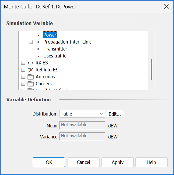
• Define variable: A Monte Carlo define variable that:
  • randomises the transmit link power
  • uses the table method
  • uses as the table the AEIRP CDF described above.

The resulting configuration is shown below.

This is clearly a much simpler simulation, but it is useful as always to test this reference system approach would give the same results.

Verification

The methodology will be checked by comparing the interference from full simulation with that using the reference system. In this example the victim will be a satellite ES.

In both simulation files the following will therefore be added:

• Antenna type: 1.2m diameter 0.6 efficiency with gain pattern Rec. ITU-R S.580-6 APL
• Station, using the ES antenna pattern and:
  • Location = 51.02°N, 0°E
  • Antenna pointing (az, el) = (180°N, 10°)
• Carrier = 180 MHz bandwidth within 200 MHz (as per creation of the AEIRP CDF)
• Link = RX link into the ES using the 180 MHz carrier, at a frequency of 26 GHz and receiver noise temperature = 150K
• Interference path from either the three 5G / IMT-2020 links or the reference system using carrier overlap as the bandwidth adjustment factor.

The propagation model from the interferers (i.e. either the 5G / IMT-2020 three links or reference system) should be set to be P.452 at 50% of time and delta N = 45.

The scenario should be to gather I/N statistics with a bin size of 0.1 dB and 100,000 samples.

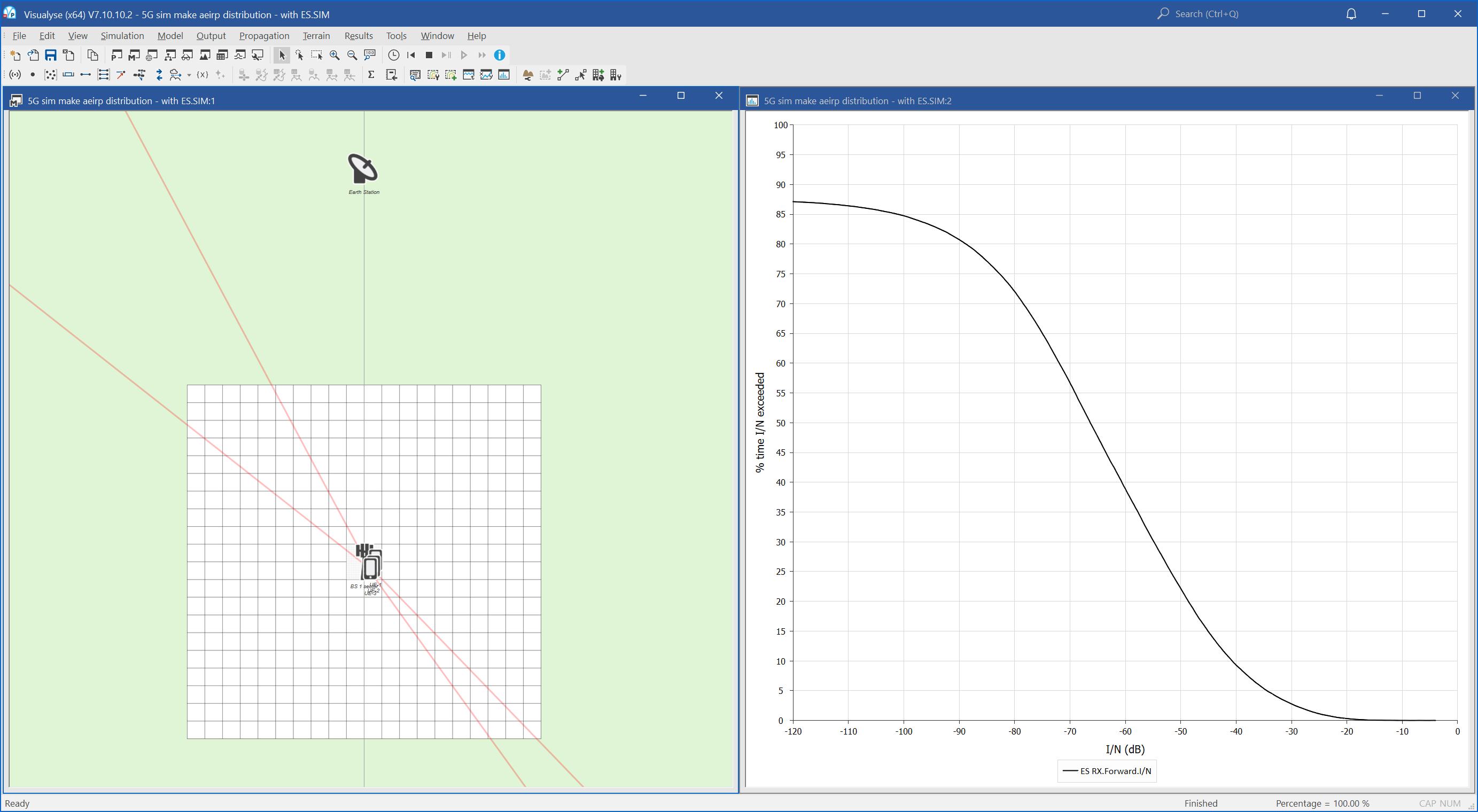
The screen shots of the two simulation files are shown below.

Full simulation:

Reference Systems Simulation:

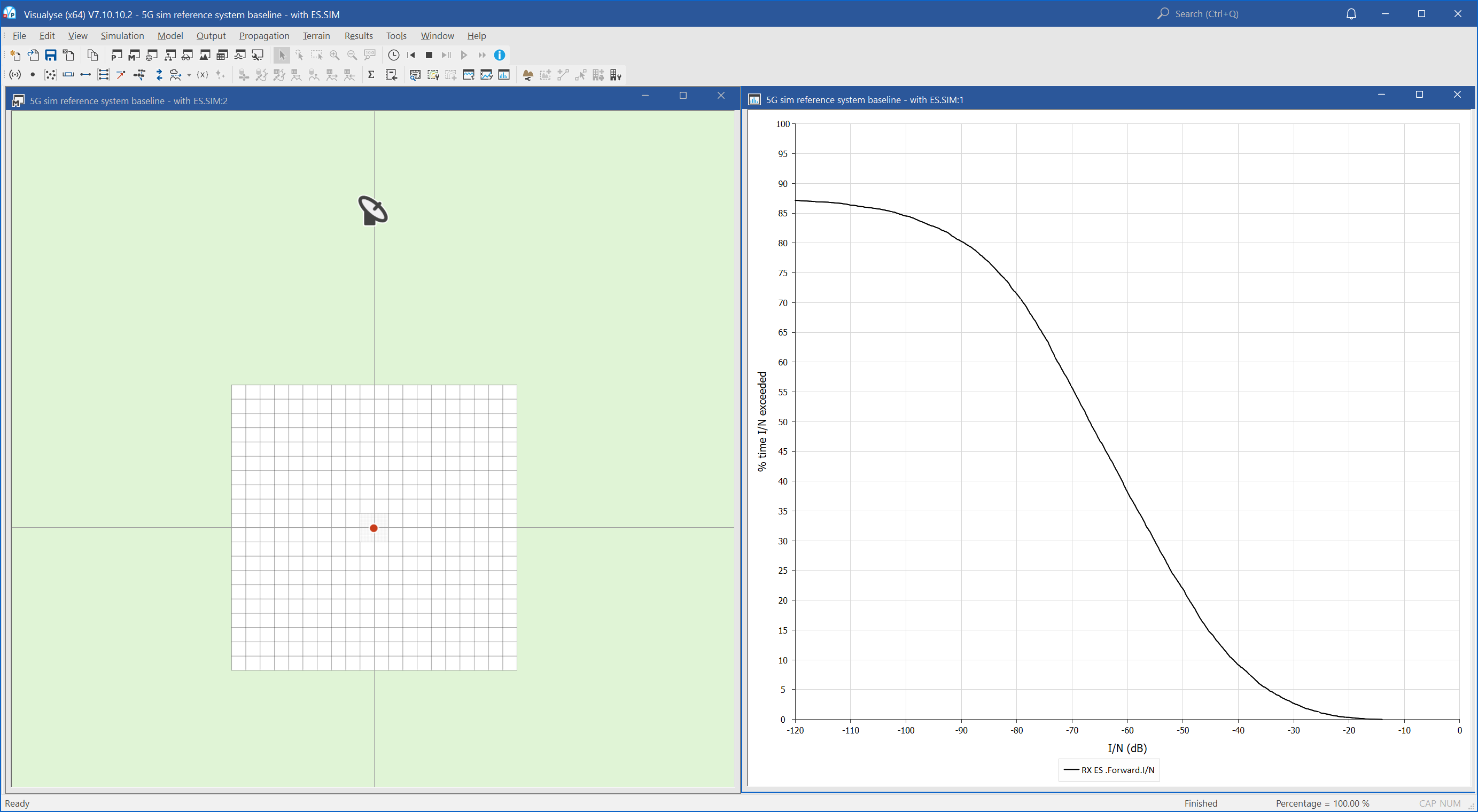
The two I/N plots look very similar. Further analysis was undertaken by exporting both CDFs to Excel as in the plot below:

It can be seen that there is good agreement between the two methods.

Developing the Model

Having created a file with a single reference station it is possible to extend it by having multiple reference stations around the ES. In addition, the propagation percentage of time can be randomised to do a full Monte Carlo analysis.

In the screen shot below there are 30 BS within a 1 x 1 km square, their locations randomised at each Monte Carlo sample:

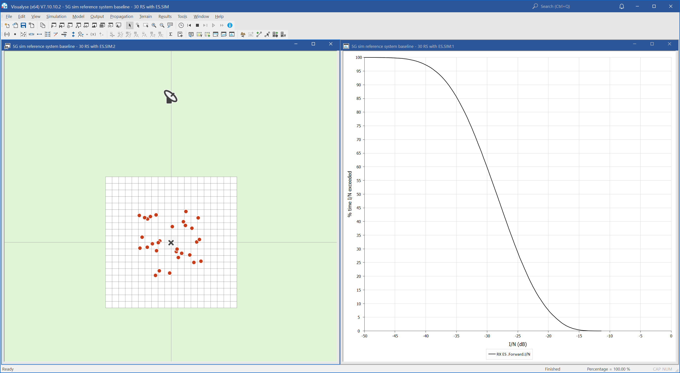
The impact on the I/N CDF compared to a single reference system can be seen in the plot below:

It can be seen that there has been a slight increase in the highest I/N and a more significant change to the rest of the CDF.

This analysis could be extended to include more reference systems modelling a wider 5G / IMT-2020 deployment all around the victim ES.