
20
Oct
Abstract
Two of the Agenda Items (AIs) at the forthcoming World Radiocommunication Conference 2023 (WRC-23) meeting relate to the operation of Earth Stations in Motion (ESIMs), namely AI 1.15 and AI 1.16. One of the issues to address under these AIs is the protection of terrestrial services and Resolution 169 (WRC-19), contains PFD limits that aeronautical ESIMS must meet to ensure that protection. This Technical Note (TN) describes how it could be verified that an aeronautical ESIMS meets these PFD limits using analysis undertaken with either Visualyse Professional or Visualyse Interplanetary.
Introduction
Requirements for the provision of broadband services to users on aircraft has led to a regulatory framework for ESIMs, whereby aeronautical stations operate within the Fixed Satellite Service (FSS) while in motion. Typically, a standard FSS Earth Station (ES) would be located at ground level at a fixed location and the regulatory framework had to be modified to take account of mobile operation and at a greater altitude. In particular, operation at this height leads to much greater distances over which there could be harmful interference, and operation on aircraft could lead to transmissions in international airspace rather than within the jurisdiction of a single administration.
Resolution 169, approved at WRC-19, covers “Use of the frequency bands 17.7-19.7 GHz and 27.5-29.5 GHz by earth stations in motion communicating with geostationary space stations in the fixed-satellite service”. The uplink bands of 27.5 – 29.5 could also be used by terrestrial stations in the Fixed and Mobile Services and protection is covered by this Resolves (amongst others):
1.2.2 transmitting aeronautical and maritime ESIMs in the frequency band 27.5-29.5 GHz shall not cause unacceptable interference to terrestrial services to which the frequency band is allocated and operating in accordance with the Radio Regulations, and Annex 3 to this Resolution shall apply;
Part II of Annex 3 to Resolution 169 contains the following PFD masks for aeronautical ESIMS:
3.1 When within line-of-sight of the territory of an administration, and above an altitude of 3 km, the maximum pfd produced at the surface of the Earth on the territory of an administration by emissions from a single aeronautical ESIM shall not exceed:
where θ is the angle of arrival of the radio-frequency wave (degrees above the horizon).
3.2 When within line-of-sight of the territory of an administration, and up to an altitude of 3 km, the maximum pfd produced at the surface of the Earth on the territory of an administration by emissions from a single aeronautical ESIM shall not exceed:
where θ is the angle of arrival of the radio-frequency wave (degrees above the horizon).
Resolves 1.2.5 of Resolution states that:
1.2.5 for the application of Part II of Annex 3 as referred to in resolves 1.2.2 and 1.2.4 above, BR shall examine the characteristics of aeronautical ESIMs with respect to the conformity with the power flux-density (pfd) limits on the Earth’s surface specified in Part II of Annex 3 and publish the results of such examination in the BR IFIC;
But how is that examination to be undertaken?
Analysis Methodologies
A Preliminary Draft New Recommendation (PDNR) is under development within WP 4A with the intention of providing a methodology by which the BR could examine the characteristics of aeronautical ESIMs (A-ESIM) to determine if they conform to the PFD limits in Annex 3 of Resolution 169. While this work is still ongoing, a useful document is the Report of the Correspondence Group (CG) on this topic in document WP 4A/883. This document also contains a draft methodology in Annex 3. The approach taken in this document is to work backwards from the PFD to the maximum EIRP that would be consistent with these limits, taking into account A-ESIM parameters such as:
- Antenna peak gain
- Gain pattern
- Carrier bandwidth
- Carrier power density
- GSO satellite longitude.
The analysis considers factors such as gaseous attenuation calculated using Rec. ITU-R P.676 and fuselage attenuation.
An alternative approach would be to calculate the PFD on the ground from an A-ESIM and compare it with the PFD thresholds for the relevant elevation angle = , and this approach is consistent with the calculation engine in Visualyse Professional and Visualyse Interplanetary and so is used in this TN.
The starting point is a simplified scenario as shown in the figure below:

In this analysis:
- An A-ESIM is operating at a height of h km above sea level
- The A-ESIM has an antenna that is pointing at its minimum elevation angle in the direction of the test point
- The A-ESIM antenna has a peak gain and gain pattern
- The A-ESIM carrier has defined (frequency, bandwidth, transmit power)
- The A-ESIM antenna is at the top of the aircraft and there can be fuselage loss towards points on the ground
- The PFD and elevation angle = is calculated at a test point and compared against the thresholds in Resolution 169 for an A-ESIM at height = h
- The geometry between the A-ESIM and test point is varied to check a range of elevation angles from 0° to 90°.
The PFD() is calculated as follows:
Where:
= transmit power in dBW in the A-ESIM carrier, with bandwidth less than the 14 MHz reference
= peak gain at A-ESIM in dBi
= relative gain at A-ESIM towards test point in dB
= fuselage loss at A-ESIM in dB
= gaseous attenuation calculated using Rec. ITU-R P.676 in dB
= spreading loss from A-ESIM to test point in dB
= distance from A-ESIM to test point in metres
The spreading loss can be calculated using:
The next section describes how this analysis can be undertaken using Visualyse tools.
Analysis in Visualyse Tools
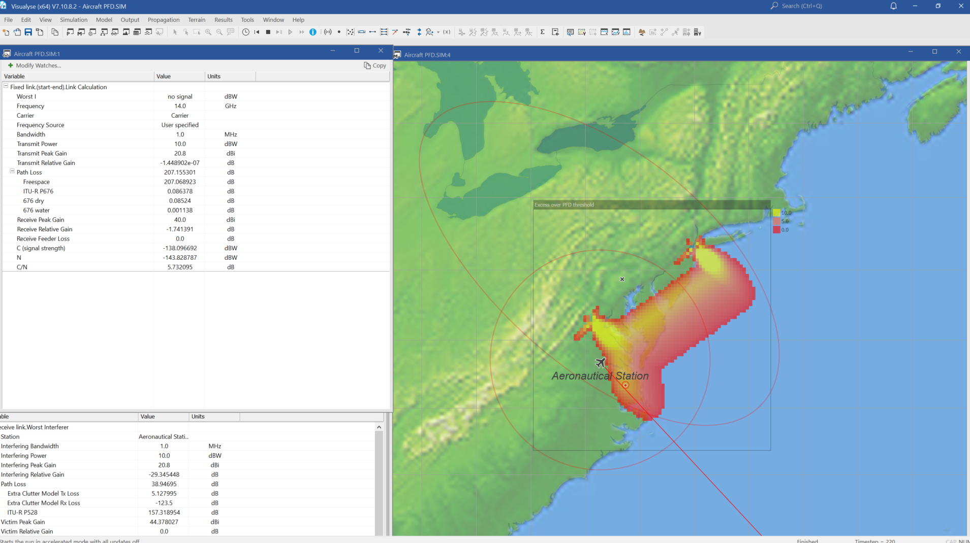
Calculation of PFD vs Elevation Angle
Visualyse can be used to calculate PFD vs. the elevation angle at which it is being received. One way to do this is shown in the simulation file shown in the figure below:
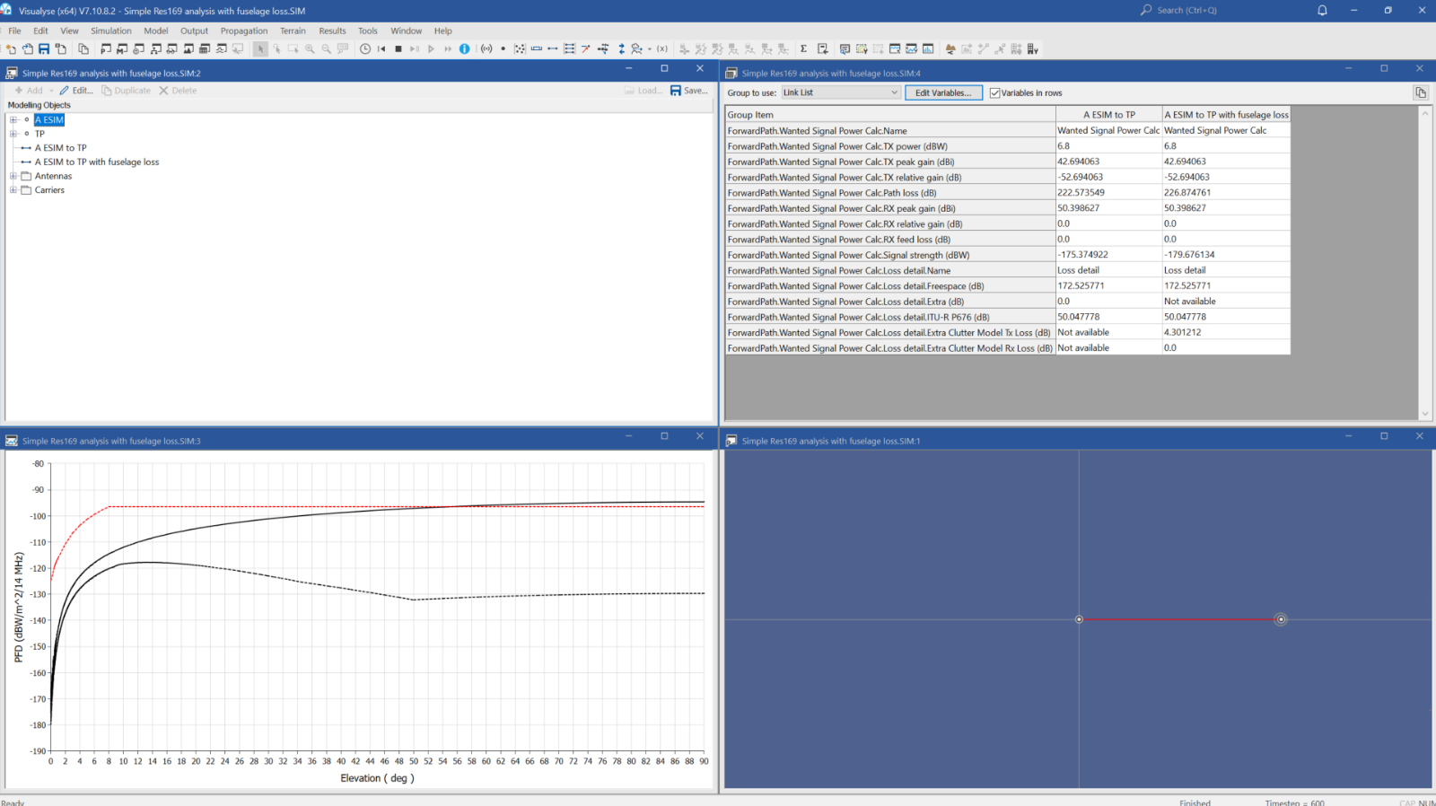
The simulation contains the following elements:
A-ESIM
- Aeronautical Station located at a (lat, long) = (0°, 0°) and height of 10 km with an Antenna pointing at an (az, el) = (90°, 20°), where 20° is assumed to be the minimum elevation angle
- Antenna Type using the gain pattern in Rec. ITU-R S.580 with dish size 0.6m and efficiency of 0.6
Test Point
- Mobile Station located at a (lat, long) = (0°, 0°) and moving in direction 90° with speed 10m/s using an Antenna pointing at the A-ESIM
- Antenna Type using the PFD Area gain pattern which converts the wanted signal into a PFD
Link-1
- From the A-ESIM to Test Point
- Carrier = 6 MHz
- Power = -61 dBW/Hz 6.8 dBW in the carrier bandwidth
- Propagation model = free space path loss plus Rec. ITU-R P.676
Link-2
- As for Link-1, but adding the fuselage loss model described below.
The run was 600 time steps of 1 minute and the following windows were opened:
- Model view to show the components of the simulation
- Map view to show the location of the A-ESIM and test point
- Table view showing the link budget calculations
- Plots of PFD vs elevation angle for the two cases, Link-1 and Link-2, compared against the Resolution 169 PFD limits (defined via a Marker array).
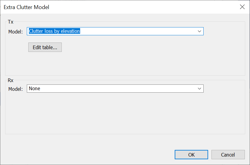
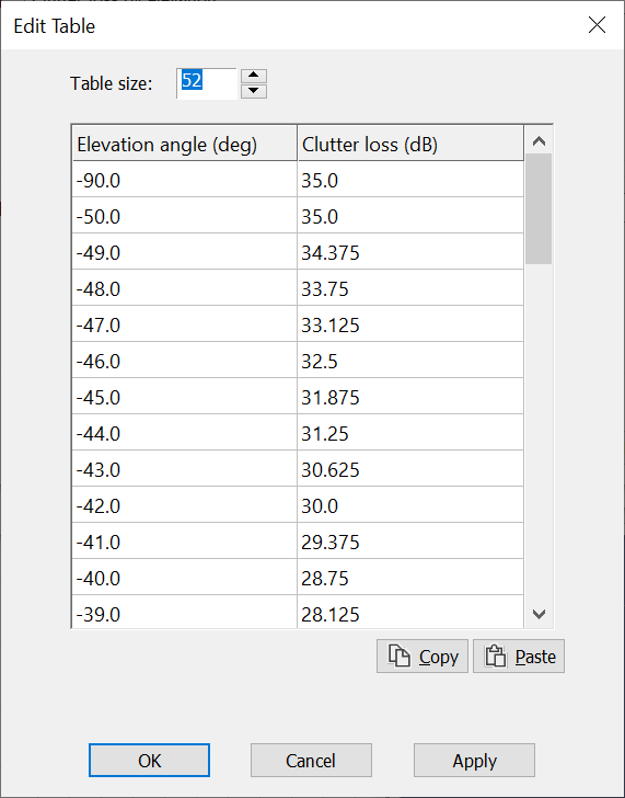
The fuselage attenuation model was the following:
This was modelled in Visualyse by including an elevation dependent clutter loss (i.e. we make use of the “Clutter loss by elevation” model to define the elevation angle dependent fuselage attenuation required here) as in the figures below:
The resulting PFD vs elevation angle for the two cases are shown in the figure below:
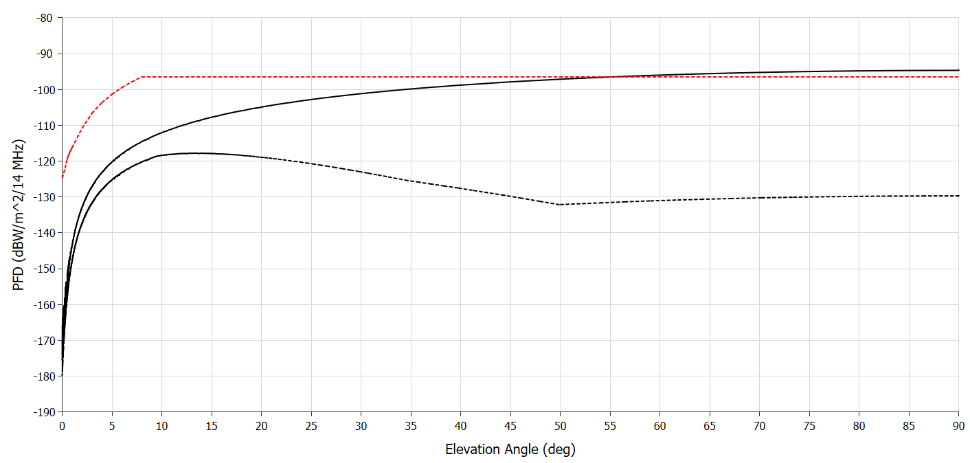
It can be seen that the Resolution 169 PFD limits are exceeded at high elevation angles in the case where no fuselage loss is included (solid line) but met for all elevation angles when fuselage loss is included (dashed line).
This approach could be automated to check many configurations in a filing (e.g. A-ESIM gain patterns, beamwidths, powers) by using the Visualyse text file format and batch mode.
Calculation of PFD over an Area
In the example above, the gain pattern was the same in all azimuths, hence its only necessary to calculate how the PFD varies by elevation. However, in some circumstances the PFD can vary by azimuth and elevation – for example, there could be asymmetric gain patterns or a non-GSO system could have a minimum elevation angle that varies by azimuth.
In this case it is possible to calculate the PFD over an area and then display the results using the Area Analysis tool. One point to consider is how to show the results, as simply plotting PFD won’t be sufficient as the threshold varies by elevation angle. One way to handle this in Visualyse is to add an elevation angle dependent clutter loss that is the same as the PFD threshold, and hence the wanted signal i.e. the PFD plotted is actually the margin compared to the Resolution 169 thresholds.
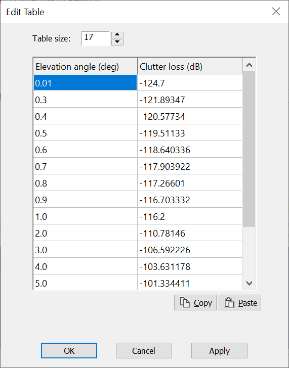
An example elevation dependent clutter table is shown below:
Area PFD Plots for an A-ESIM communicating with a non-GSO System
Consider the case of an A-ESIM communicating with a non-GSO constellation using a beamforming antenna. This could result in PFDs that vary in azimuth and also elevation as beamforming antennas can generate gain patterns that are not monotonically decreasing. The resulting PFD depends upon the positions of the satellites and the various sidelobes of the beamforming antenna, and hence can vary over time. To get the maximum PFD possible at each location it is therefore necessary to undertake a simulation over multiple time steps and constellation configurations.
In the example below, where the antenna is modelled using Rec. ITU-R M.2101, the A-ESIM’s PFD margin against threshold is shown for a single time step, where an A-ESIM located on the equator is communicating with a satellite towards the south-west:
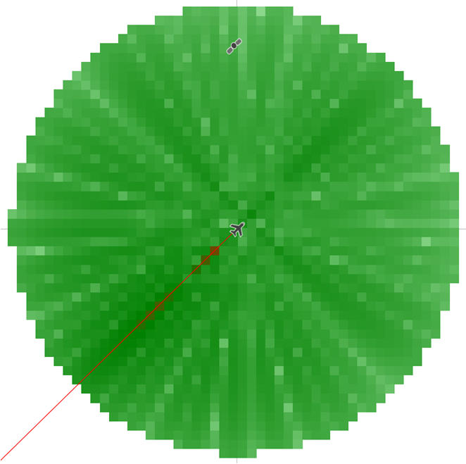
The peaks and troughs of the M.2101 gain pattern can be seen around the A-ESIM, and a zone of higher PFD in the direction of transmission.
This analysis can be repeated for many different constellations positions to determine the highest PFD at each pixel of the Area Analysis (AA) after one-thousand time steps, as shown in the figure below:
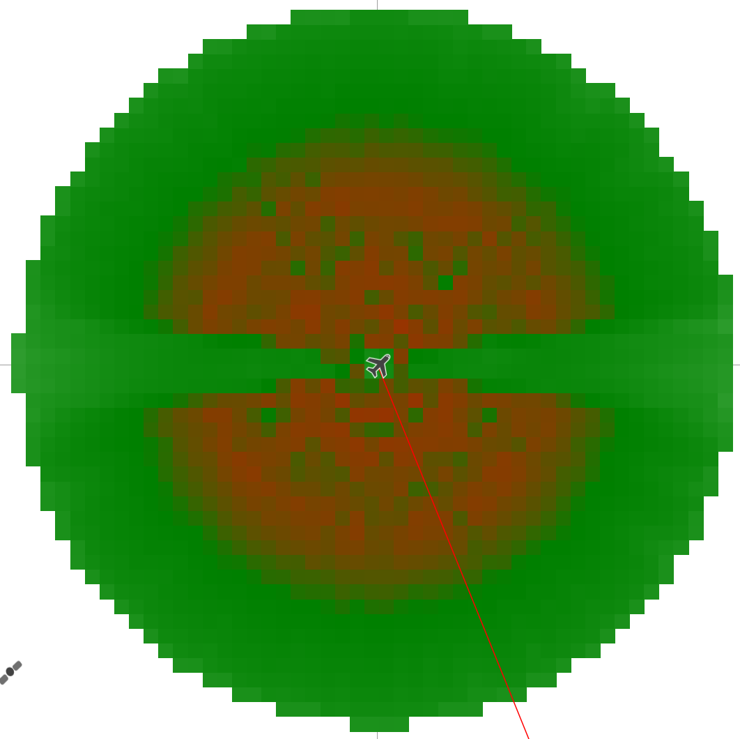
The PFD margin over threshold can be seen to be lowest (and possibly over) for a range of elevation angles, but with a distinct zone in the middle where the PFD is much lower. This zone reflects the GSO arc exclusion zone, as the A-ESIM cannot point towards a non-GSO satellite that could result in its antenna also pointing towards the GSO arc. In this case the A-ESIM is on the equator, so the exclusion zone is along the east-west line below the aircraft. The geometry of this zone varies by latitude, so the PFD analysis might have to be repeated multiple times.
Area PFD Plots for an A-ESIM Travelling along a Coastline
This Area Analysis approach would also allow the modelling of the maximum PFD margin over an area such as a seaboard as an A-ESIM flies along the coastline. An example of this is shown below:
Use in Visualyse Interplanetary
Note that these features are available in both Visualyse Professional or Visualyse Interplanetary and hence could be used to analyse A-ESIMs features around other celestial bodies, for example as part of regulatory regime for aircraft flying on Mars!
Consultancy Support
We can also use our Visualyse tools to undertake studies relating to ESIMS for ITU-R studies and to support regulatory and licensing activities.