
12
Jan
Abstract
Recommendation ITU-R RS.2017 defines thresholds that can be used as interference criteria when undertaking studies of interference into Earth Exploration Satellite Service (EESS) (passive) systems. This Recommendation defines the threshold in terms of a threshold interference level and a percentage of a reference area that the interference level into a receiver may be exceeded. The threshold interference level, size of reference area and maximum percentage are defined for a range of frequency bands between 1.37 and 956 GHz. This Technical Note (TN) describes ways to model these thresholds in Visualyse Professional.
Introduction
Satellites operating under the EESS (passive) service are vital to understand and monitor the Earth. They provide information that can be used for a wide range of applications including weather forecasting, monitoring and understanding global warming and tracking changes in land use. As a passive service it is measuring natural phenomena that can require high sensitivity to pick up weak signals, which can make it susceptible to harmful interference.
This sensitivity can make it difficult to share co-frequency with active services, and indeed Article 5.340 identifies that all emissions are prohibited in a set of frequency bands. Often, therefore, sharing scenarios are non-co-frequency, between an active service in one band and the EESS (passive) in another.
These types of sharing scenario can be modelled in Visualyse Professional, including complex new technologies such as 5G and mega-constellations of non-GSO satellites.
A key step is to be able to compare the interference levels calculated with the thresholds in Recommendation ITU-R RS.2017. These thresholds are defined based upon areas on the surface of the Earth. For example, in the 23.6 – 24 GHz band this would be:
- Reference bandwidth = 200 MHz
- Threshold interference level T(I) = -166 dBW
- Percentage of area that T(I) maybe exceeded = 0.01 %
- Reference area = 2,000,000 km2
The question is then, how to model this type of threshold in Visualyse Professional?
Example Scenario
To demonstrate how to model this type of threshold, an example scenario will be considered that has:
- EESS (passive) operating below 24 GHz
- 5G / IMT-2020 deployment above 24 GHz
Note that the parameters used are not agreed but are examples to demonstrate the methodology.
5G/IMT-2020 Parameters
The 5G example parameters were based upon document 5D/TEMP/265-E rev 3.
The starting point was the definition of a single site with a base station (BS) and three UEs. The approach used to create the basic simulation is described further in the TN: Building a 5G Network in Visualyse Professional.
The questions are then how to model:
- A widescale deployment of 5G systems across the reference area of 2,000,000 km2?
- The non-co-frequency scenario?
The deployment was derived from the following parameters:
- Percentage of area where 5G systems are deployed = 5%
- Percentage of deployed area that is dense-urban = 10%
- Density of BS in non-dense-urban areas = 10 BS/km2
- Density of BS in dense-urban areas = 30 BS/km2
The percentage of area within which 5G systems are deployed = 5%, which implies an area of 100,000 km2 or a square 316 x 316 km. Within this deployed area there could be 1,200,000 BS. This is too many for each one to be modelled individually.
There are multiple ways to model large deployments in Visualyse Professional, including:
- Model large numbers of transmitters: while accurate this can lead to large simulations that are slow to update
- Model a limited number of transmitters in detail and derive the EIRP cumulative distribution function (CDF) and use that as the input to a larger simulation. More information is available in the TN: Building a 5G Reference System in Visualyse Professional
- Use simplifying methods, such having N actual systems being modelled by 1 simulated system and then increasing the power by 10log10(N). Care is required in this approach that there are enough simulated systems modelled to capture the range of configurations feasible.
The approach taken was to have 120 5G systems in the model, each representing 10,000 actual 5G systems and scale the power by 40 dB.
The second question is then how to model non-co-frequency scenarios. Again, there are a number of methods in Visualyse Professional:
- Define the transmit and receive spectrum masks and undertake a detailed analysis by integrating the two masks to calculate the mask integration adjustment (sometimes called the NFD)
- Specify the BS / UE power directly from the power density in the victim bandwidth and set the interferer frequency equal to the victim frequency
- Calculate the difference between co-frequency and non-co-frequency power density and adjust the interfering signal accordingly.
In addition, there are a number of ways of defining how the gain pattern in Recommendation ITU-R M.2101 varies in the frequency domain.
The approach used here was to take a power density in the adjacent band of -42 dBW/200 MHz. The in-band BS power density was calculated to be -9.7 dBW/60 MHz which means the adjacent band levels are 37.5 dB below the in-band levels.
With an aggregation factor of 40 dB and taking off 3 dB for polarisation mismatch loss, the consequence was that the scenario was modelled with 120 5G systems and an aggregation factor of -0.5 dB.
EESS (Passive) Parameters
Parameters for EESS (passive) systems between 1.4 and 275 GHz are given in Recommendation ITU-R RS. 1861. This typically gives a range of characteristics and sensor F2 was used in this case with parameters:
- Altitude = 705 km
- Inclination = 98.2
- Peak gain = 46.7 dBi
- Beamwidth = 0.9
The gain pattern was taken to be that in Recommendation ITU-R RS.1813.
A key factor to model is the how the sensor is pointed at the spacecraft, and options include:
- Nadir scan
- Conical scan
- Push-broom.
In this case we will consider both nadir and conical scan options.
Defining the Reference Area
The reference area could be any location on Earth and the study is intended to be generic, not dependent upon actual country or cities. A more specific study could be done using population data, as described in the TN: Using Population Data in Visualyse Professional.
For a generic study, all that is required is a latitude and in this case a value of 40N was assumed. An area of 2,000,000 km2 equates to a square with side 1,414.2 km which can be modelled as 12.7 of latitude and 16.6 of longitude.
Modelling Methodologies
This scenario can be modelled in a number of ways, most importantly:
- Dynamic: modelling the orbital motion of the satellite
- Monte Carlo: convolving the various input parameters to derive statistical outputs.
The first approach considered was dynamic.
The propagation model for the interfering path was free space path loss, gaseous attenuation using P.676 and clutter loss using P.2018 (elevation dependent loss).
Dynamic Analysis
In dynamic analysis, the position of the EESS satellite is calculated using an orbit propagator. The question is then: how to ensure that statistics are only collected when the satellite is taking measurements in the reference area?
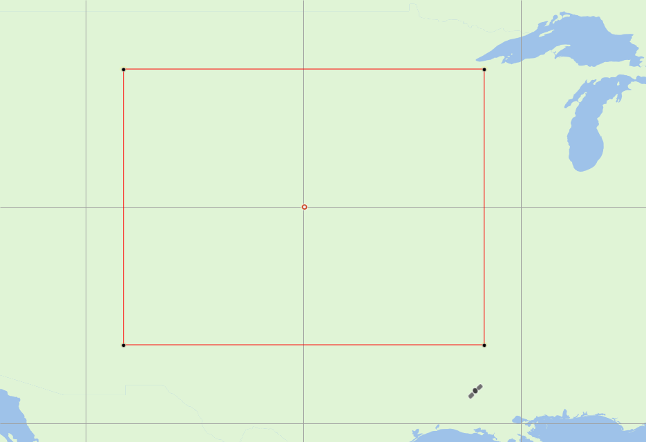
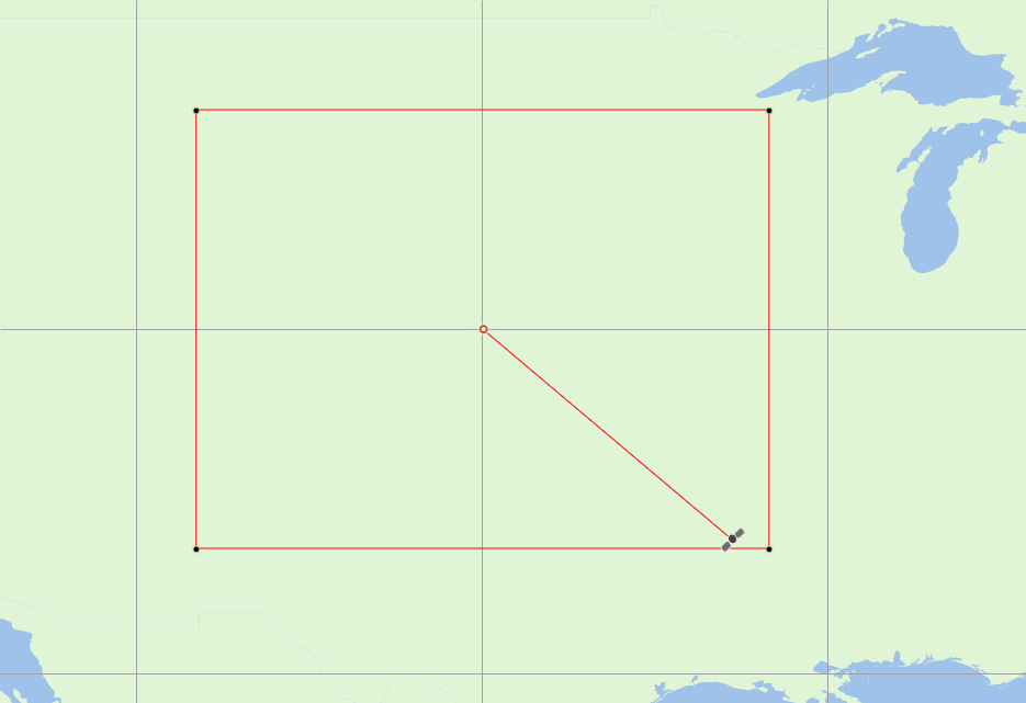
For the nadir case, this can be done using a tracking strategy using the following approach:
- Create a control Station at the centre of the reference area
- Create an empty Station Group and put the EESS non-GSO satellite in it
- Create a Tracking Strategy that checks that the difference in latitude and longitude is less than that for the reference area
- Create a Dynamic Link starting at the control Station and ending at the EESS Station Group using the Tracking Strategy
Then the link will only be active when the EESS satellite is within the reference area. Hence the statistics created will refer to those measurements only.
The link can be seen to switch on when inside the box in the following screenshots:
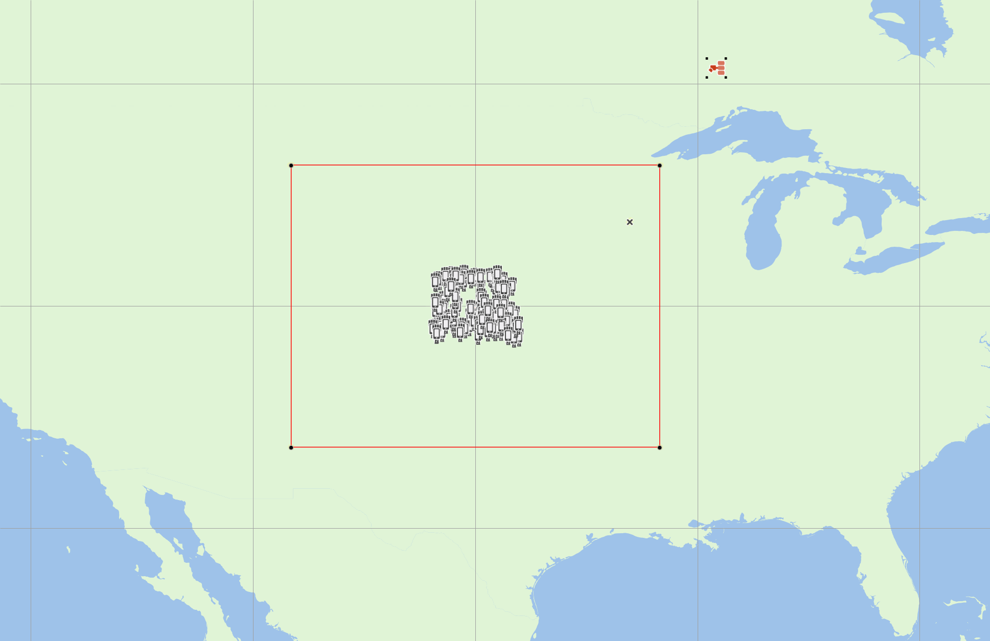
When the 5G systems are added the complete SIM looks like this:
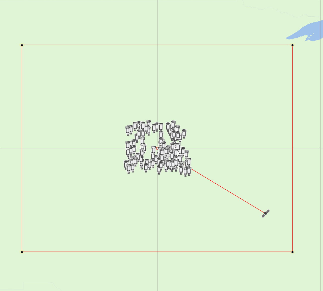
Note the clustering of all 5G systems in a single location might be considered to be a pessimistic assumption.
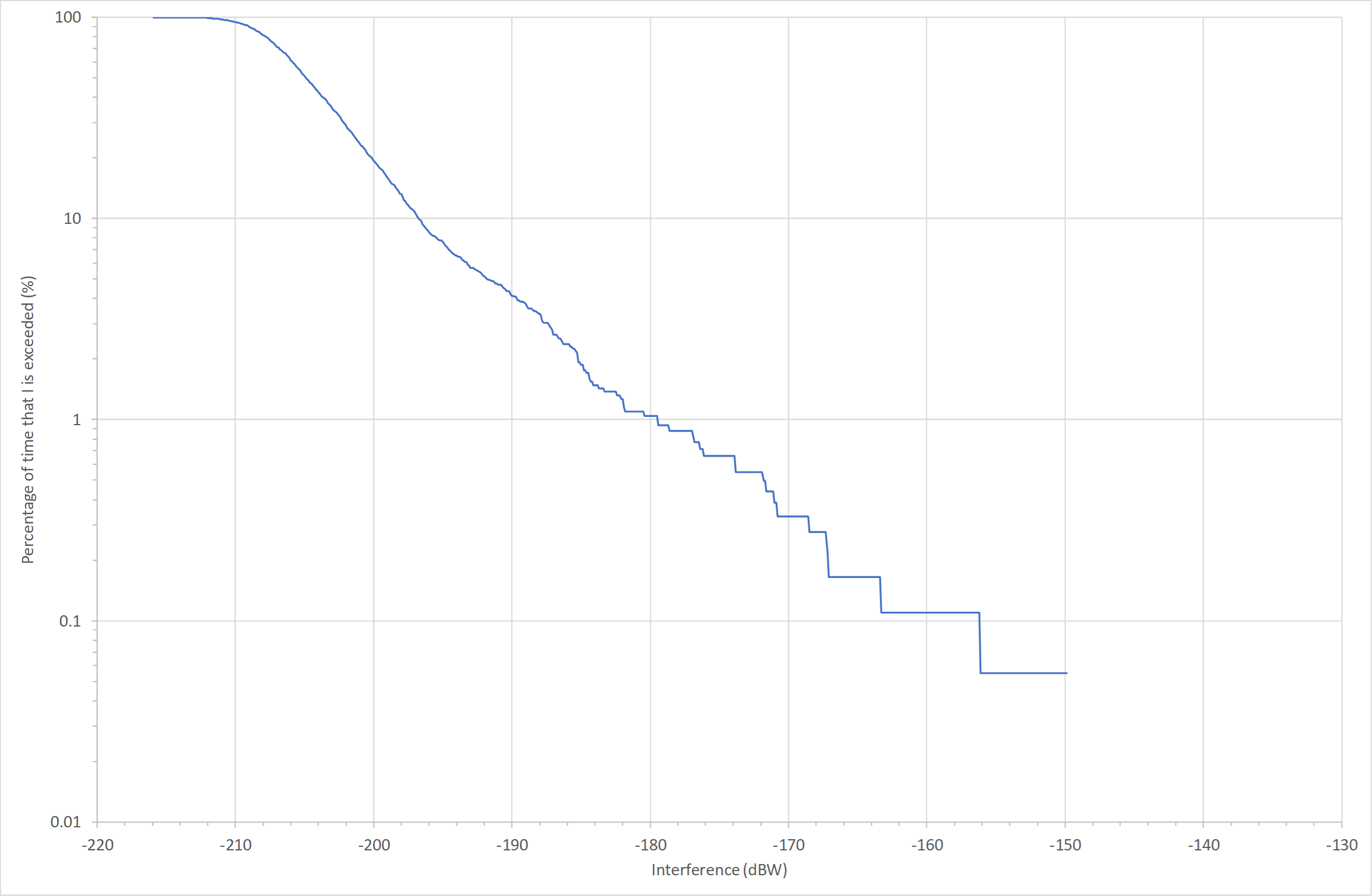
The simulation was run for 1 month with time step 5 seconds and the resulting CDF of the interference was follows:
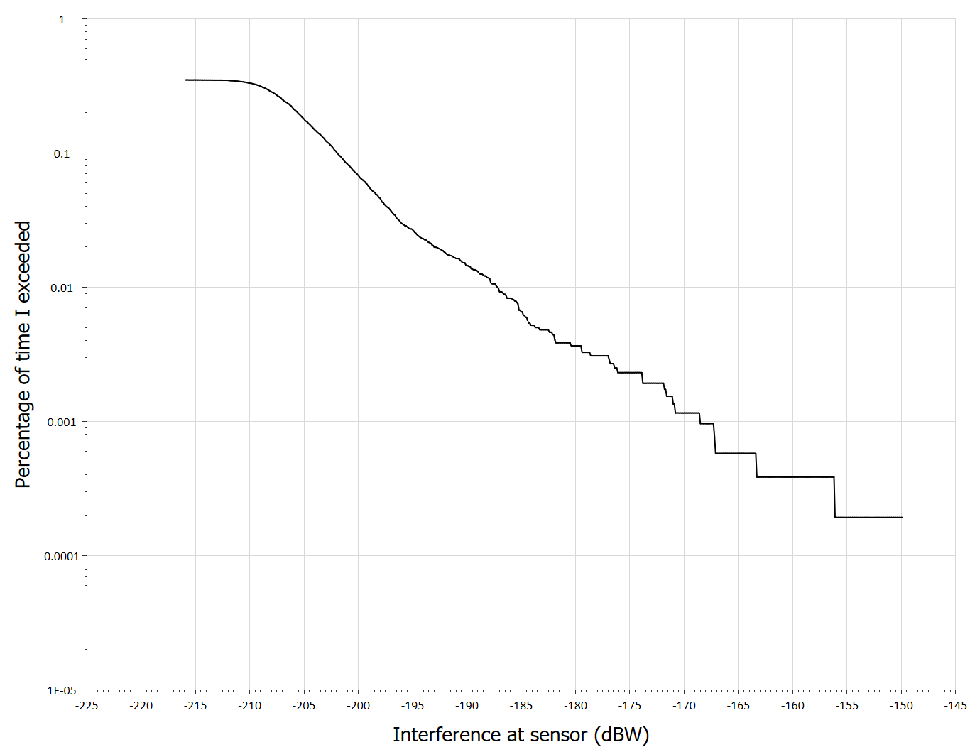
Two things can be noticed about this plot:
- At small percentages of time, the CDF is not a smooth curve but shows a series of steps. For scenarios such as this, where interference is into an antenna with parabolic main beam, the small percentages of time part of the curve should be parabolic, whereas here the last segment is a horizontal line. These two facts suggest that further time steps are required.
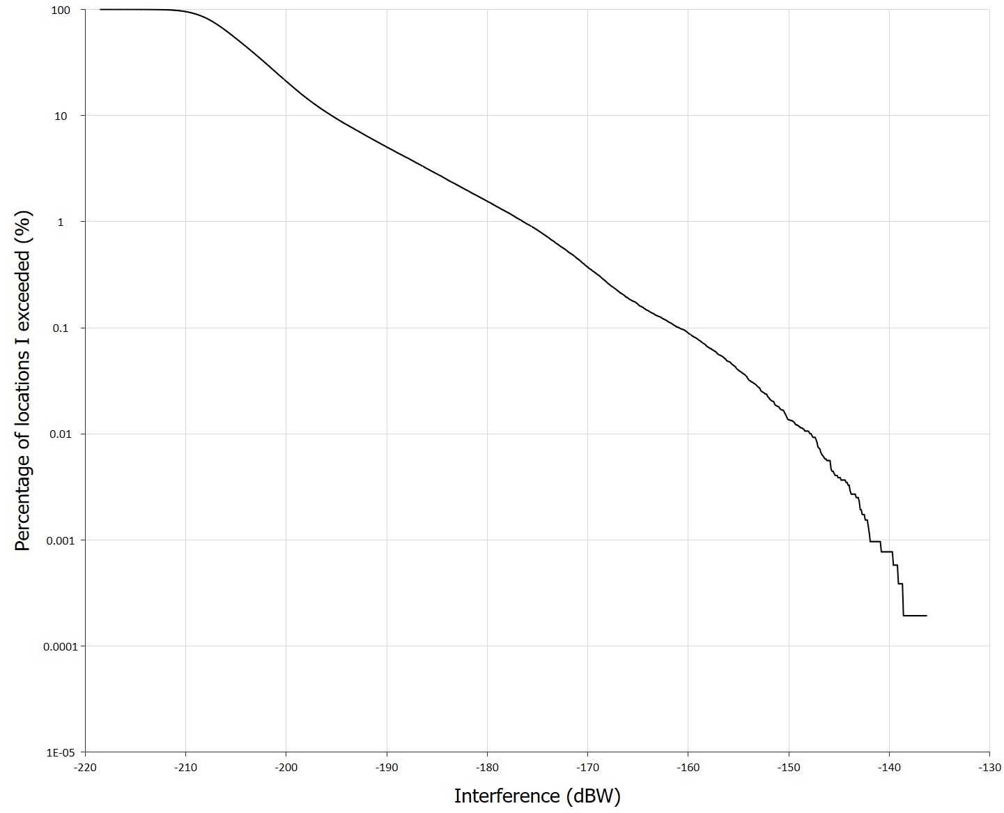
- The CDF does not go up to 100% but has a maximum percentage of 0.35%. This is because the link was only active when the satellite was in the reference area. The data must therefore be normalised to when the link is active, resulting in the following plot:
It can be seen that the threshold is exceeded.
This approach isn't very computationally efficient as for the majority of time steps (over 99% of them) the simulation is updated but the satellite is outside the reference area.
An alternative approach is to use Monte Carlo methods to directly model the satellite at a random position within the reference area, as described in the following section.
Monte Carlo Analysis
In this approach, the satellite location is defined via (latitude, longitude) which is then randomized to be within the reference area. This approach is more efficient as each time sample is used to generate statistics, rather than only 0.35% of them. It also allows more flexible pointing methods, as discussed in the following section.
Care is required to ensure the propagation models such as P.676 use the Earth-space path classification, which can be done by enabling the slant-path calculation option. In addition an extra trans-horizon loss must be added to ensure 5G stations beyond line of sight of the EESS satellite are not included. The antenna pointing must also be modified for the reference frame with elevation set to -90°.
Having done this the simulation can be run for the same number of samples as the dynamic analysis and the following CDF generated:
Note that:
- The curve is the same as that for dynamic analysis for high percentages of time
- The curve is smoother (and hence likely more accurate) for low percentages of time.
- No normalization is required, as the statistics are already over the reference area.
This approach also allows analysis of other sensor pointing methods, as in the following sub-section.
Modelling a Conical Sensor
A conical sensor scans at a fixed angle from the line to the sub-satellite point. This can be modelled by:
- Creating a test point to be the sensor boresight location
- Randomizing this test point within the reference area
- Randomizing the location of the EESS (passive) satellite at a fixed distance from this test point and random azimuth
- Pointing the EESS (passive) antenna at the test point.
The distance from the test point to the EESS (passive) satellite is a function of the pointing angle and satellite altitude. In this case an angle at the satellite = 47.5° was used which corresponds to a distance of 830.7 km.
The simulation can be seen in this screenshot:
The resulting CDF is shown in the figure below:
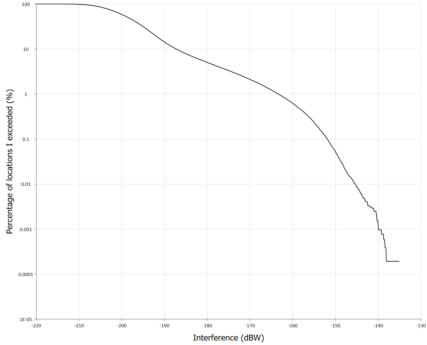
Interference at the 0.01% of locations exceeded the -166 dBW threshold by about 21 dB. If the -166 dBW aggregate threshold was apportioned by 3 dB, the result was an exceedance of about 24 dB.
These numbers are consistent with the contents of the CPM-19 Report to WRC-19, as described in section 2/1.13/3.2.1.2.1.
Developing the Model
This model could be further extended in a number of ways:
- Changing the deployment with alternative clustering of 5G cells
- Including time of day variations in 5G traffic levels
- Modelling alternative EESS (passive) sensors
- Including more 5G cells in the simulation (and reducing the aggregation factor)
- Using alternative methodologies, including reference systems
- Including indoor systems and indoor-outdoor loss
- Modelling the behaviour of the M.2101 gain pattern in the adjacent band and including a normalisation factor
- Using alternative parameters to model the 5G emissions including power in adjacent bands
- Manufacturing margin etc.
Conclusion
This TN has shown ways to model in Visualyse Professional interference into EESS(passive) systems using the reference area interference metric in Recommendation RS. 2017.
Two approaches were considered, one based upon dynamic simulation and the other on Monte Carlo methodologies. Two different sensors were modelled, one using nadir pointing and the other conical.
The results were CDFs of the interference into the EESS (passive) sensor. All input parameters were examples, though results generated were similar to those presented in the CPM-19 Report.