
11
Oct
Abstract
A key component of any satellite system are the Earth Stations (ES). These must be licensed and this regulatory process varies between countries and frequency bands. One common technique is to define a threshold in terms of a power flux density or PFD and for the ES operator to have to derive the contour which shows those locations where the PFD would be exceeded. In some cases there can also be a requirement to identify the population that would be within this PFD contour. This Technical Note (TN) looks at how this information can be generated using Visualyse Professional.
Introduction
A number of methods have been identified to facilitate the introduction of satellite Earth stations (ES) in bands shared with other services. One example is the approach used in the United States in the 27.5 – 28.35 GHz band to share with stations of the Upper Microwave Flexible Use Service (UMFUS).
The requirement in the FCC’s Section 25.136 is to identify the area where the ES generates a PFD at 10 m above ground level of greater than or equal to -77.6 dBm/m2/MHz. The requirement is that the population within this area should be no more than 450 people.
This Technical Note (TN) describes how to model this scenario in Visualyse Professional and derive the metrics required.
There are two approaches to consider, depending upon whether the ES emissions are constant in time or vary. These can be summarised by the two cases:
- Static, such as for a GSO satellite ES transmitting using a constant power
- Dynamic, such as for a non-GSO satellite ES with antennas that track as the satellite moves overhead
These two cases are handled separately below.
GSO Satellite Example
Parameters
The ES parameters for this example are given below:
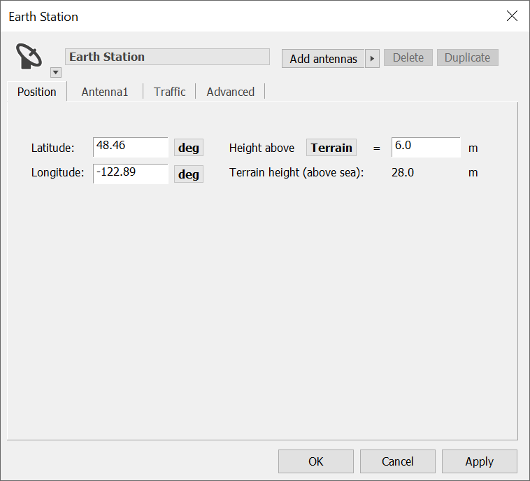
- Latitude = 48.46466°N
- Longitude = -122.8868°E
- Antenna height = 4 m
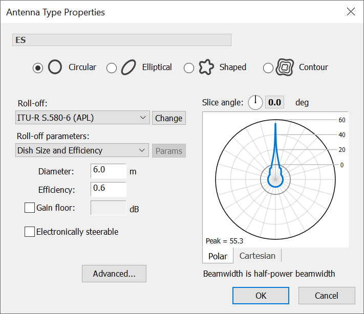
- Antenna diameter = 6 m
- Transmit power = -18 dBW/MHz
- Antenna gain pattern = Rec. ITU-R S.580 APL
If measured antenna gain data is available that should be used as this will lead to more accurate results.
The satellite is assumed to be located at 93°W.
Creating the Antenna Types and Stations
The dialogs of the ES Antenna Type and Station are shown in the following two figures:
As well as creating Stations for the ES and GSO satellite, it is also necessary to create a test point to measure the PFD.
This should be a Terrestrial Station with height = 10m, as per the requirement in Section 25.136.
To make it easier to derive PFD in Visualyse Professional the test point should use an Antenna Type with the “PFD Area” as shown in this figure:
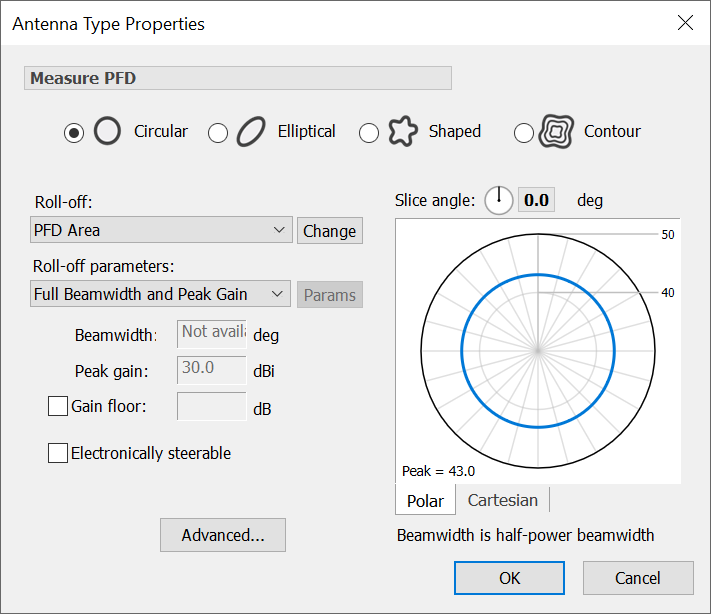
This creates an Antenna Type with peak gain in all directions equal to the effective area of an isotropic antenna, namely:
Using this gain means that the signal received is equal to the PFD using:
This is required as the "standard" PFD in Visualyse Professional is calculated using the Article 21 assumption of free space path loss, via:
Creating the Carriers and Links
The Carrier can be a default one with bandwidth 1 MHz.
The polarisation has an impact on the propagation loss calculated so should be selected carefully. In this case we’ll consider linear horizontal.
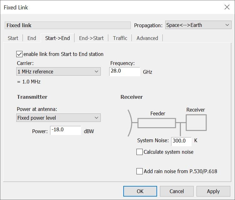
Then a Fixed Link can be created:
- Start Station = Earth Station
- End Station = Test Point
- Propagation Environment = Earth to Space
- Frequency = 28 GHz
- Carrier = 1 MHz Reference
- Transmit power = -18 dBW
The Start->End direction dialog is shown below:
Propagation Environment
This is a critical step and the models used should be chosen carefully.
One propagation model that is often chosen for these types of study is the one in Recommendation ITU-R P.452. This can be configured to take account of local geoclimatic conditions including the Delta N and N0.
Typically the PFD contours are very close to the satellite ES, and for these short distances there is only a small variation in propagation loss. Hence it can be acceptable to use a long-term percentage such as 50%. However if the contour is large then it could be necessary to consider short-term variations.
The resulting dialog is similar to that below:
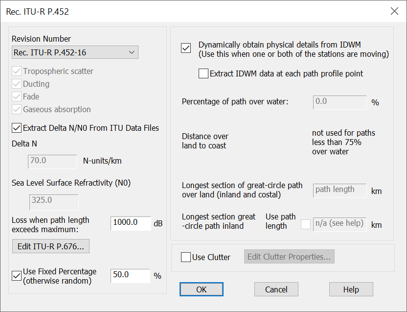
Note that this does not currently include clutter loss which is discussed later.
Creating the PFD Contour
Having created the simulation this way, using the PFD Area Antenna Type, then the wanted signal of the Fixed Link will be the PFD to be displayed.
This PFD can be shown across an area using the Area Analysis tool configured so that:
- The Station that is moved is the PFD Test Point
- The parameter to be displayed is the Fixed Link wanted signal C (i.e. the PFD)
The threshold is Tr(PFD) = -77.6 dBm/m2/MHz which in dBW is -107.6 dBW/m2/MHz.
On the Area Analysis this can be shown graphically and can be coloured in red or brighter yellow using:
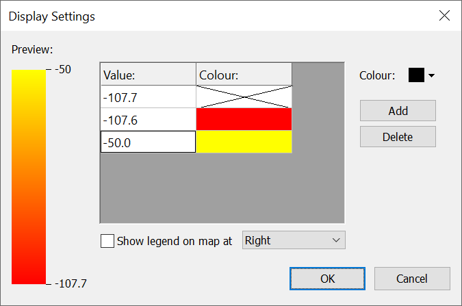
It can require some iteration to find the right size of the Area Analysis and pixel size. It is generally better to start with a large area with big pixels and make the size of the area and pixels smaller as the scales become clearer to the user through iteration.
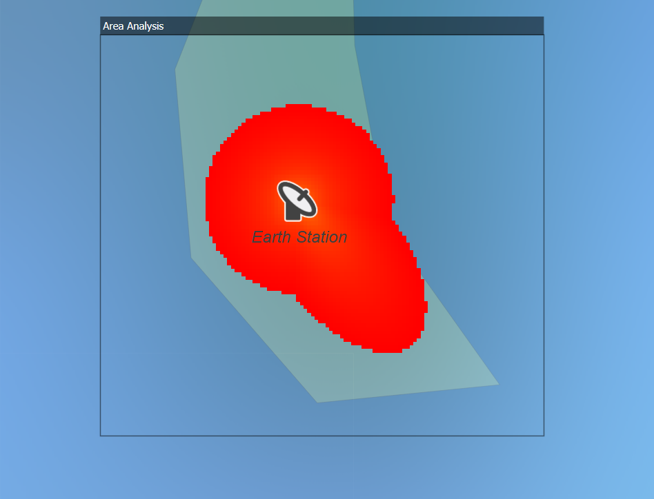
At this stage there is no terrain, so the resulting contours will be smooth, like this:
Terrain Data
The next stage is to include the effects of terrain. A number of terrain databases might be available: in general, the higher the resolution the more likely it is to be accurate.
Hence it is better to use (say) the 30 m Shuttle Radar Topography Mission (SRTM) data than the equivalent 90 m data.
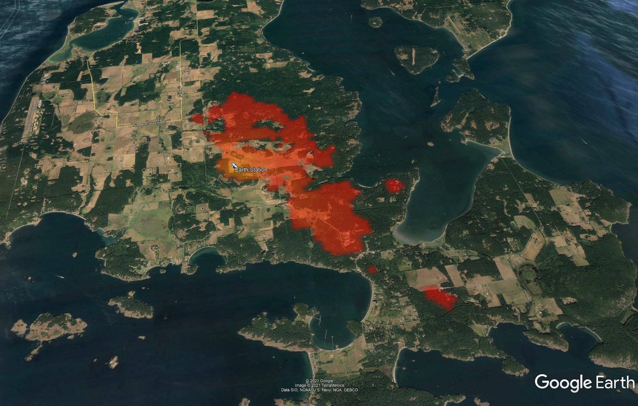
The impact of using 90 m resolution SRTM data is shown in the figure below:

It can be seen that the impact of considering terrain is to significantly reduce the size of the contour.
This area can be visualised by exporting to Google Earth, as in the figure below:
Population Data
The Visualyse Professional population data tool can then be used to identify the number of people within this effected area.
More information about this feature is available in a separate Technical Note, but the key steps are:
- Download the population data from the Transfinite web site
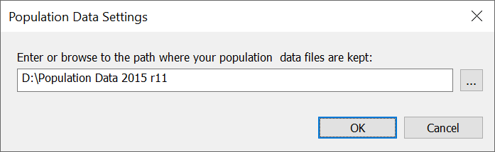
- Select the directory with the population data in the File|Population Data Settings dialog:
- On the Area Analysis, right click and then select the “Export Population Data” option.
This will generate a CSV file with the population within each of the levels specified to show the PFD. In this case the output was:
| Range | Population |
|---|---|
| < -107.7 | 1293 |
| -107.7 to -107.6 | 0 |
| -107.6 to -50.0 | 95 |
| > -50.0 | 0 |
It can be seen that the population effected would be 95, which is below the threshold of 450 identified in FCC’s Section 25.136.
Impact of Clutter
This level of modelling could be sufficient to allow the ES to be authorised. But in some cases the population within the contour could be above 450. In this case additional mitigation could be considered, in particular the impact of clutter.
Clutter loss could be due to existing obstructions such as buildings and trees near the ES, or it could be the result of a new structures built as site shielding.
These can be included in the simulation using one of the clutter models, including that within ITU-R P.452. In this case the parameters can be entered using this dialog:
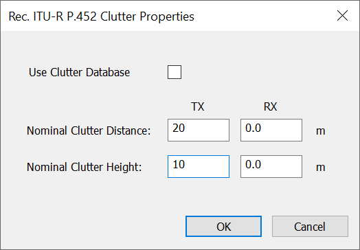
Note that the receive end could be anywhere within the Area Analysis and hence there could be a range of distance to clutter and height of clutter. If a land use database is available it could be used to determine the nominal clutter distance and height to use at the transmit and/or receive ends.
Other clutter models could be used, including P.2108, though it is not clear which of these would be applicable as:
- Height-gain model: this is only applicable up to 3 GHz
- Statistical clutter model: this is designed for Monte Carlo modelling for paths over 250m in urban or suburban environments
- Ground to air or space model: this is not designed for terrestrial paths.
Another approach is to determine the clutter loss using external tools or measurement and then enter the value directly as an “Extra loss”.
Modelling non-GSO Satellite ES
Modelling non-GSO ES can be more complicated as the ES antenna pointing changes as the satellites move overhead, and hence the gain towards the test point is not a static value.
A number of approaches could be used, including:
- An initial approach could be to determine the maximum gain towards the horizon and then use that as the gain pattern using the same Area Analysis approach as for the GSO ES
- A more advanced approach could use an area Monte Carlo methodology that convolves the antenna pointing at the non-GSO ES (and possibly transmit power control) with propagation variation. This would use the alternative Advanced Contouring method.
More information about these approaches is available on request.